Pendulum Inverse Identification with JAX

How do you figure out the physical constants of a system when all you have are noisy measurements? This post walks through using JAX to solve an inverse problem: learning the damping and gravitational constants of a pendulum from observed angle data.

The Problem

The second-order ODE for a damped pendulum is:

where $b$ is the damping coefficient and $c$ is related to gravity and pendulum length. We want to learn $b$ and $c$ from measurements of $\theta(t)$.

To use JAX’s ODE solver, we convert this to a first-order system by defining angular velocity $\omega(t) = \theta'(t)$:

Setting Up the Model

First, the imports and the ODE system:

import jax.numpy as np
from jax import jit, random, value_and_grad
from jax.experimental.ode import odeint


def pend(y, t, b, c):
    theta, omega = y
    return np.hstack([omega, -b * omega - c * np.sin(theta)])


def model(y0, t, params):
    return odeint(pend, y0, t, *params)

Generating Synthetic Data

In practice you’d have experimental measurements. Here we simulate them with added noise:

# True parameters
b = 0.25
c = 5.0
true_params = np.asarray([b, c])

# Initial conditions: nearly vertical, at rest
y0 = [np.pi - 0.1, 0.0]

# Time points
t = np.linspace(0, 10, 101)

# Simulate and add noise
data = model(y0, t, (b, c))
theta, omega = data.T
key = random.PRNGKey(0)
noisy_theta = theta + 0.3 * theta * random.normal(key, shape=theta.shape)

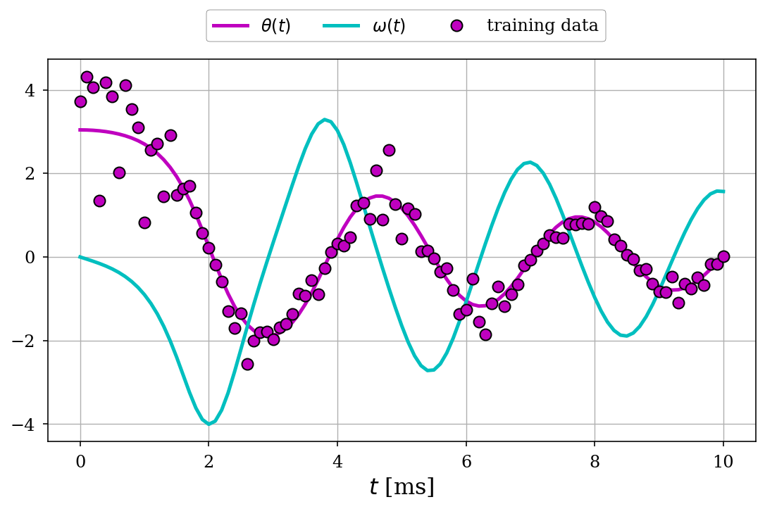
The plot below shows the true dynamics (angle $\theta(t)$ in magenta and angular velocity $\omega(t)$ in cyan) along with the noisy training data (magenta dots):

Learning Parameters with Gradient Descent

The key insight: JAX can differentiate through the ODE solver. We define a loss function and use value_and_grad to get both the loss and its gradient with respect to parameters:

def mse(y_true, y_pred):
    return np.mean((y_true - y_pred) ** 2)


@jit
def loss_fn(params, y0, t, y_true):
    y_pred = model(y0, t, params)
    return mse(y_true, y_pred[:, 0])


@jit
def step(params, y0, t, y_true, lr):
    loss, grads = value_and_grad(loss_fn)(params, y0, t, y_true)
    return params - lr * grads, loss

Then we run gradient descent:

# Random initial guess
key, subkey = random.split(key)
params = random.uniform(subkey, shape=(2,), minval=0, maxval=10)

# Training loop
lr = 0.01
for epoch in range(1000):
    params, loss = step(params, y0, t, noisy_theta, lr)
    if epoch % 100 == 0:
        print(f"Epoch {epoch}, Loss: {loss:.6f}")

opt_params = params

Results

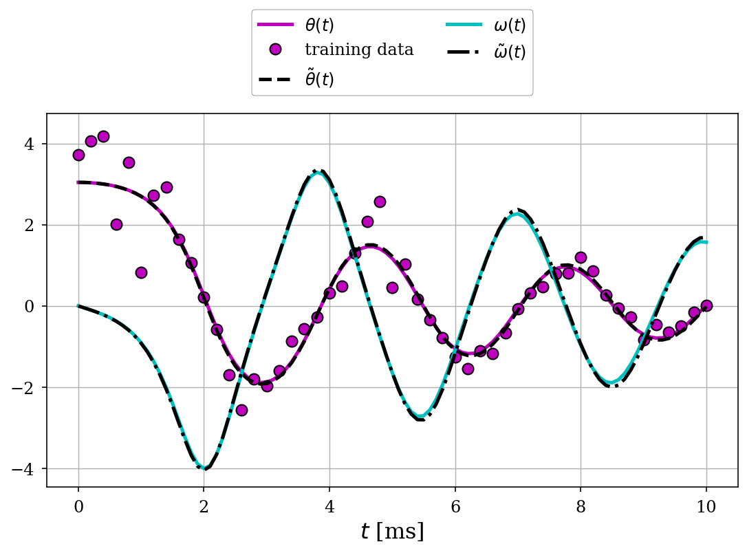
After training, the fitted parameters closely match the true values:

              Actual | Initial | Fitted
b (damping):   0.25  |  3.42   |  0.26
c (gravity):   5.00  |  7.81   |  4.98

The fitted trajectory (dashed black lines) matches the true solution almost perfectly, recovering the underlying dynamics despite measurement noise:

Why This Matters

This approach, differentiating through a physics simulator, is powerful. You can:

• Learn physical constants from real-world data
• Calibrate simulation parameters
• Do system identification without deriving analytical gradients

JAX makes this almost trivial. The same pattern works for much more complex systems: neural ODEs, PDE solvers, anything you can write as a differentiable program.