Computer graphics papers often carry the same baseline numbers from one comparison table to the next. This is reasonable because reproducing every established method would consume time better spent evaluating the proposed contribution. It also leaves an interesting question unanswered. How much headroom remains in a mature baseline if it receives sustained attention from an agentic research loop?
This study explores that question through point-cloud surface normal estimation, continuing earlier work on smoothing splines and adaptive neighborhood selection. The PCPNet benchmark is a useful case because PCA has remained a standard reference across years of normal-estimation papers. Its published average angular RMSE is 16.25°. The learned PCPNet method reports 14.58°, while the recent state of the art, PFF-Net, reports 9.38°.
Starting from fixed-neighborhood PCA, 322 agent experiments were run through a protected scientific harness. The resulting approach achieved 14.36° average RMSE on the complete official PCPNet test protocol. It reduced error by 11.7% relative to a same-harness PCA baseline and slightly outperformed PCPNet, without training data or a learned model.
This does not make a PCA-derived method the new state of the art. PFF-Net remains 4.98° better on average. The result instead shows that a familiar baseline contained enough geometric headroom to cross a meaningful published reference once persistent experimentation became cheap enough to attempt.
The Standard PCA Baseline Still Has Slack
The standard PCA estimator is compact. For each query point, gather its $k$ nearest neighbors, compute their covariance matrix, and return the eigenvector associated with the smallest eigenvalue. The resulting vector is the normal of the least-squares local plane.
Its weaknesses are also well established in the literature. A large neighborhood averages positional noise but blurs curvature and sharp features. A small one preserves local detail but produces a noisy covariance estimate. Uneven sampling shifts the effective center of the patch, while points from another surface sheet can exert disproportionate influence.
Those problems admit many geometric responses, including distance weighting, robust residual losses, different supports for estimating scale and covariance, repeated plane refinement, and confidence gates between local scales. Choosing and combining them is the difficult part. The final method is therefore more sophisticated than the short phrase “tuned PCA” suggests, even though PCA remains its computational foundation.
The earlier spline and adaptive-neighborhood studies reached the same broader theme from two directions. Smoothing splines showed that an analytical surface fit can be competitive when the geometry is modeled explicitly. Adaptive neighborhoods showed that a globally fixed scale wastes information available in the local eigenstructure.
The question here was whether an agent could repeatedly formulate, implement, measure, reject, and refine such ideas while the evaluation protocol remained under human control.
Building the Phased Agentic Research Loop
The phased agentic development workflow was developed by my team at Infobip as a structured way to operate coding agents across research, planning, task definition, and implementation. Its premise is that decisions made before coding shape everything downstream, so each phase produces a curated artifact for the next one. Four context operations keep the agent focused across the phases. Evidence is written outside the conversation, relevant context is selected, completed work is compressed into curated artifacts, and independent tasks are isolated in fresh sessions.
For this experiment, that structure was combined with Andrej Karpathy’s autoresearch approach. The evaluator stays fixed while an agent edits one method, the result is measured, improvements are retained, and the process repeats. Karpathy’s project applies this idea to autonomous experiments on single-GPU language-model training. Its original setup asks one long-running agent session to keep experimenting. Here, that process was moved into an outer controller. Every experiment ran in a fresh agent process, while canonical records, concise notes, and Git state carried research knowledge forward.
Figure 1 summarizes the resulting design. The phased workflow fixes the research protocol, while the outer loop repeats bounded experiments in fresh sessions.
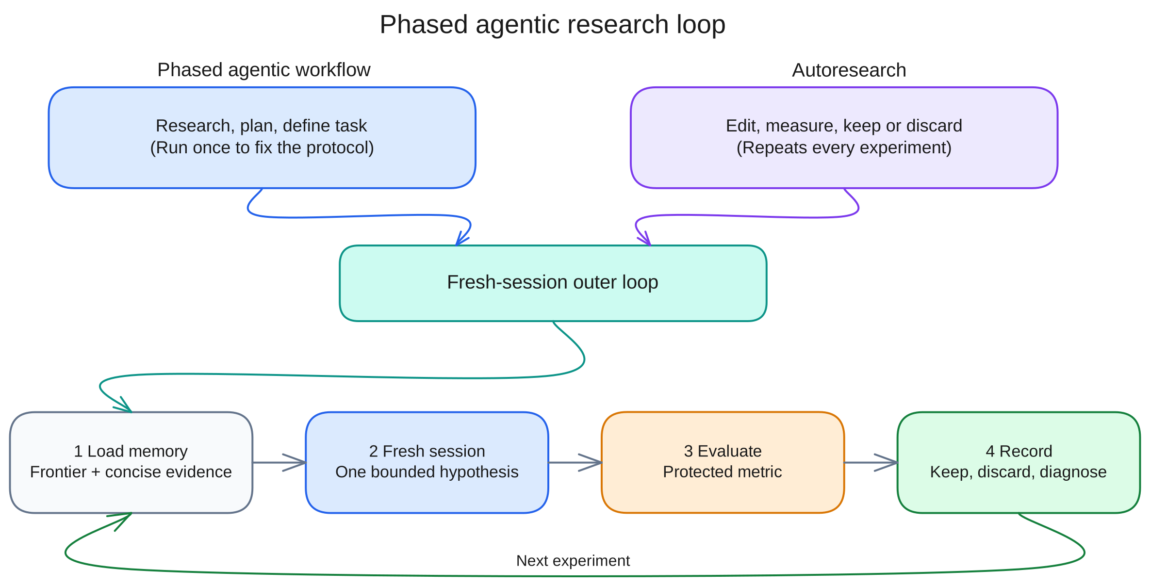
The phases were performed once to define the research protocol. The outer loop then repeated the implementation phase and used each result to generate the task context for the next attempt.
| Phase | Decision made before or during the study | Durable artifact |
|---|---|---|
| Research | PCPNet protocol, prior methods, leakage risks, geometric constraints | README and references |
| Planning | development, validation, and test tiers, acceptance thresholds, simplicity rules | controller policy |
| Task definition | one geometric hypothesis and one independently removable change | iteration instructions and proposal schema |
| Implementation | isolated edit, formatting, evaluation, rollback, and recording | estimator commit and canonical record |
The phased workflow and the outer loop complement each other. The workflow prevents the agent from redefining the problem while optimizing it. The loop makes it affordable to examine hundreds of small hypotheses after the protocol is fixed. Canonical records store evidence. Path-scoped tools select what each session sees, regenerated summaries compress finished work, and a disposable workspace isolates every attempt.
The research agent ran in Pi, a minimal, extensible terminal coding harness that can run interactively or as a process embedded in another workflow. Pi supplied the model with controlled file-editing tools and allowed the outer controller to start a new non-interactive process for each attempt. GPT-5.6-sol was configured with high reasoning. The search ran for just under 18 hours, during which the controller launched 322 fresh agent sessions. API token counts and monetary cost were not persisted, as noted among the limitations.
Inside the Protected Harness
A research loop needs more than a prompt and a score. If editable code can inspect labels, test data, or the evaluator itself, an apparent improvement can be leakage rather than a better method. The complete experiment implementation separates the research session, prediction process, and scorer.
Every iteration began with a disposable workspace. A fresh Pi process received copies of the current estimator, protocol, search state, aggregate result history, concise research notes, and per-condition memory. The harness exposed only two path-scoped tools. One read a small allowlist of research files. The other performed exact text replacements in estimator.py or proposal.json. No shell or general-purpose file tool was available to the agent.
The agent was asked to make exactly one explainable change. Its proposal had to identify a geometric failure mode, explain the mechanism, predict condition-level trade-offs, estimate the complexity cost, and state an independent ablation. Previous development and validation scores were intentionally available because they carried the findings of earlier sessions. Test scores, reference normals, per-shape errors, shape names, and the mapping between anonymous evaluation inputs and conditions were not available.
When the session ended, the outer controller validated the proposal and checked that the estimator was the only tracked source file changed. It then applied deterministic Ruff fixes, formatting, and linting before committing and tagging the candidate. Candidate code was evaluated only after that snapshot had been created.
Prediction and scoring were separate processes. During prediction, estimator.py received point coordinates, official query indices, and precomputed nearest-neighbor indices and distances. The prepared jobs used anonymous item identifiers. On macOS, the worker ran in a process sandbox that denied network access, blocked protected project and user paths, limited CPU time and memory, and allowed writes only to the prediction directory. The worker could produce normal vectors but could not read the reference normals or evaluator.
The protected evaluator then loaded the saved predictions and reference normals in a separate process. It computed per-shape angular RMSE, aggregated the six benchmark conditions, and returned only the permitted metrics to the controller. It never imported agent-editable code. This separation prevented a candidate from adapting its output to labels or scores during evaluation.
Figure 2 shows the trust boundary and the possible outcomes of an attempt.
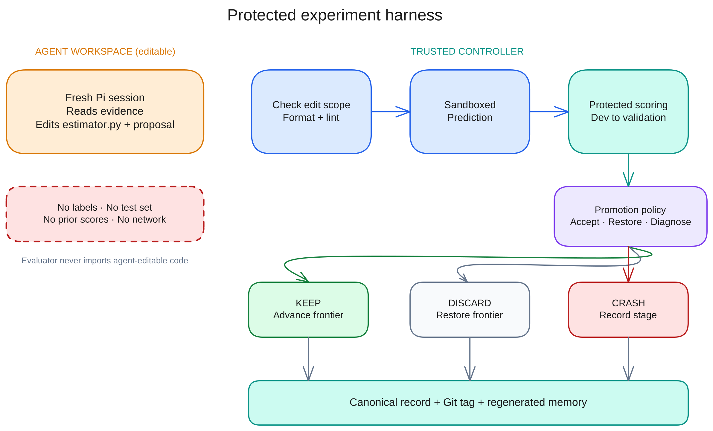
For every iteration, the controller performed the same sequence.
- It created an isolated workspace and launched a fresh agent process.
- It validated the proposal and edit scope.
- It applied deterministic Ruff fixes, formatting, and linting.
- It committed and tagged the candidate before evaluation.
- It ran sandboxed prediction and protected scoring on development data.
- It sent qualifying candidates to validation.
- It advanced the frontier, restored the previous estimator, or recorded the exact failure stage.
- It regenerated concise notes and condition memory from immutable records.
Routine development experiments had to improve aggregate RMSE by at least 0.05°. A candidate that reached validation had to improve the validated frontier by another 0.05°, unless it delivered a measured simplification. Rejected or crashed candidates could not silently replace the frontier.
Every session started without conversational history, while files and Git retained evidence from prior work. The next agent saw compact knowledge rather than hundreds of earlier transcripts. Eighteen attempts crashed and 282 were discarded, but their diagnostics and negative findings remained available to later sessions.
Measuring Progress Without Touching the Test Set
For an estimated normal $\hat{\mathbf n}_i$ and reference normal $\mathbf n_i$, the metric was sign-invariant angular error.
$$ e_i = \frac{180}{\pi}\arccos\left( \left|\frac{\hat{\mathbf n}_i^\top \mathbf n_i} {\lVert\hat{\mathbf n}_i\rVert\lVert\mathbf n_i\rVert}\right| \right). $$For shape $s$, the score is
$$ \operatorname{RMSE}_s = \sqrt{\frac{1}{N_s}\sum_{i=1}^{N_s} e_i^2}. $$PCPNet groups shapes into clean, low-, medium-, and high-noise conditions, plus stripe and gradient density variations. Per-shape RMSE was averaged within each condition, and all six conditions were then weighted equally.
Evaluation used three tiers.
- Development sampled 1,000 deterministic queries from each official training point cloud.
- Validation used every official query from the three validation geometries.
- Test used all 540,000 official queries from 108 test-list entries after the finalist was frozen.
The fast development score was only a proxy. A lower development score did not automatically become the new estimator. Validation decided the retained frontier. The complete test set was evaluated once for the frozen finalist. The original PCA implementation was evaluated afterward only to provide a controlled comparison under the same cache, runner, evaluator, and aggregation.
What 322 Experiments Found
The study produced 323 canonical records, comprising one baseline and 322 agent attempts. Of 304 measured agent candidates, 24 reached validation. Eleven changes replaced the validated frontier, giving 12 retained records including the baseline. The last retained estimator appeared at iteration 279. The remaining 43 attempts did not justify replacing it. Figure 3 shows the complete development trajectory.
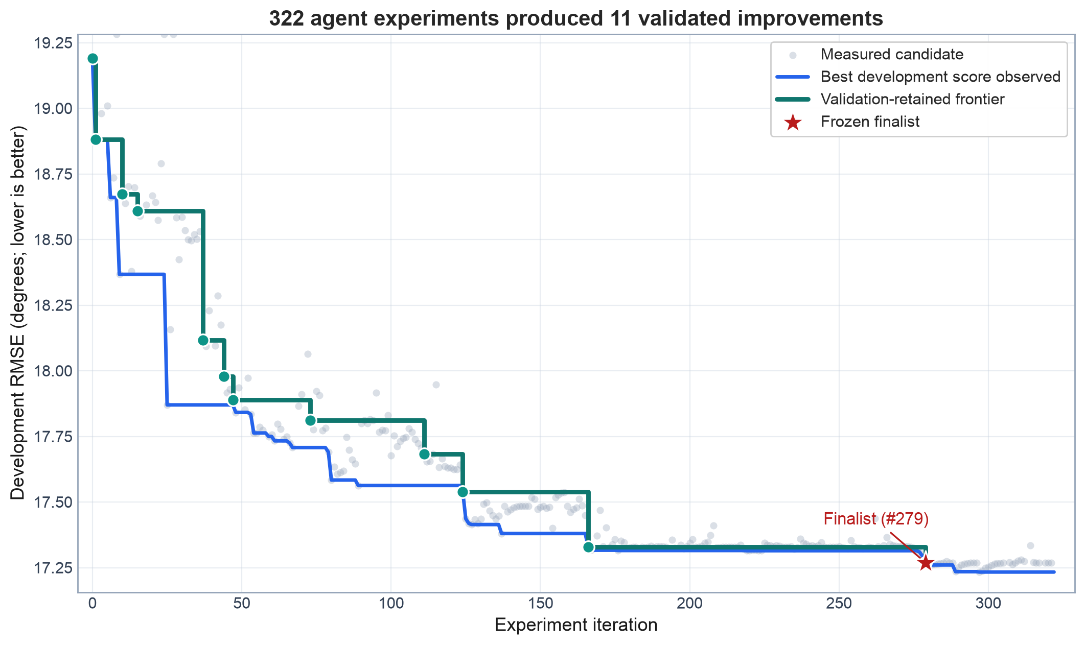
The blue line is the best development result observed, including candidates that were not retained. The teal line is the validation-backed frontier. Their divergence matters because optimizing the cheap proxy alone would have selected a different method.
The successful path was cumulative but interpretable. It moved through the following changes.
- Gaussian distance weighting instead of uniform covariance.
- One and then two robust residual-reweighting steps.
- A broad 224-neighbor initialization followed by local refinement.
- Weighted medians and median absolute deviations for residual location and scale.
- Tukey’s redescending biweight in place of Cauchy weights.
- Smaller cores for estimating robust statistics while keeping broader covariance support.
- A third refinement accepted only for geometrically thin local sheets.
- Extrapolation of the last accepted normal correction.
No single prompt invented the final method. The loop accumulated evidence. An idea improved one condition but harmed another, a parameter probe bracketed a useful range, or a rejected candidate revealed that residual thickness could not fully distinguish curvature from noise. Fresh contexts did not remove cumulative reasoning because that reasoning was stored in structured records.
The Final Estimator
The resulting approach remains local, deterministic, CPU-only, training-free, and PCA-derived. It uses broad support to reduce variance, robust local statistics to reduce geometric bias, and a gate to avoid over-refinement on noisy or strongly curved patches. It proceeds in four stages.
- Compute a Gaussian-weighted PCA normal over 224 neighbors. The distance to neighbor 112 sets the kernel bandwidth, so the outer half of the patch contributes a decaying tail rather than uniform broad support.
- Refit a plane on 112 neighbors with Tukey weights derived from point-to-plane residuals. A tighter 64-neighbor core estimates the weighted residual median and median absolute deviation those weights depend on.
- Refit again, now on 128 neighbors, but read residual location and scale from only the nearest 32. Covariance averaging keeps its broad support while the decision about what counts as an outlier uses a much more local sample.
- Compute a third robust fit and accept it only when the residual spread indicates a thin local sheet. For accepted patches, sign-align the new normal and extrapolate the latest correction by 80%. Otherwise, keep the second fit.
The spatial weight for neighbor $i$ is
$$ g_i = \exp\left[-2\left(\frac{d_i}{d_{112}}\right)^2\right]. $$For signed plane residual $r_i$, weighted residual median $m$, robust scale $\hat\sigma$, and cutoff $c$, the Tukey factor is
$$ t_i = \begin{cases} (1-u_i^2)^2, & |u_i|<1,\\ 0, & |u_i|\geq 1, \end{cases} \qquad u_i = \frac{r_i-m}{c\hat\sigma}. $$Each covariance uses normalized weights proportional to $g_i t_i$. The third fit is accepted when
$$ \hat\sigma \leq 0.1\,d_{112}. $$This gate is best understood as a residual-thickness proxy, not a perfect classifier. A compact residual distribution suggests that another redescending fit can remove geometric contamination without throwing away too much valid support. Large residual spread can come from noise, curvature, or multiple sheets, so those patches keep the more conservative second normal.
Comparison with Published Results
The table below combines representative values from the PFF-Net comparison with both PCA controls, the agent-derived approach, and a spline-based method from my earlier work. Lower RMSE is better.
| Method | None | Low | Medium | High | Stripe | Gradient | Average |
|---|---|---|---|---|---|---|---|
| Controlled fixed-$k$ PCA | 12.28 | 12.86 | 18.40 | 27.61 | 13.63 | 12.79 | 16.26 |
| Published PCA | 12.29 | 12.87 | 18.38 | 27.52 | 13.66 | 12.81 | 16.25 |
| PCPNet | 9.64 | 11.51 | 18.27 | 22.84 | 11.73 | 13.46 | 14.58 |
| Discovered approach | 9.13 | 10.43 | 18.20 | 27.18 | 11.33 | 9.89 | 14.36 |
| Zhou et al. | 8.67 | 10.49 | 17.62 | 24.14 | 10.29 | 10.66 | 13.62 |
| My spline-based method | 7.04 | 11.36 | 19.71 | 27.75 | 8.00 | 7.82 | 13.61 |
| DeepFit | 6.51 | 9.21 | 16.73 | 23.12 | 7.92 | 7.31 | 11.80 |
| AdaFit | 5.19 | 9.05 | 16.45 | 21.94 | 6.01 | 5.90 | 10.76 |
| GraphFit | 5.21 | 8.96 | 16.12 | 21.71 | 6.30 | 5.86 | 10.69 |
| MSECNet | 3.84 | 8.74 | 16.10 | 21.05 | 4.34 | 4.51 | 9.76 |
| PFF-Net | 3.32 | 8.34 | 15.63 | 20.94 | 4.10 | 3.92 | 9.38 |
The spline row reports a previously published experiment rather than a same-harness rerun. It is included to place the current result beside my earlier analytical method.
The same-harness PCA result differs from the published value by 0.01°, which confirms the protocol reproduces the reference. Against that control, the discovered approach drops the average by 1.90°, from 16.26° to 14.36°. It also moves below PCPNet by 0.22°. PCPNet remains much better under high noise, while the discovered approach gains most on clean data and uneven density.
A paired nonparametric bootstrap over shape entries, stratified by condition, gives a discovered-approach-minus-baseline average difference of -1.90°, with a 95% interval of [-2.23°, -1.59°]. Figure 4 shows the condition-level intervals.
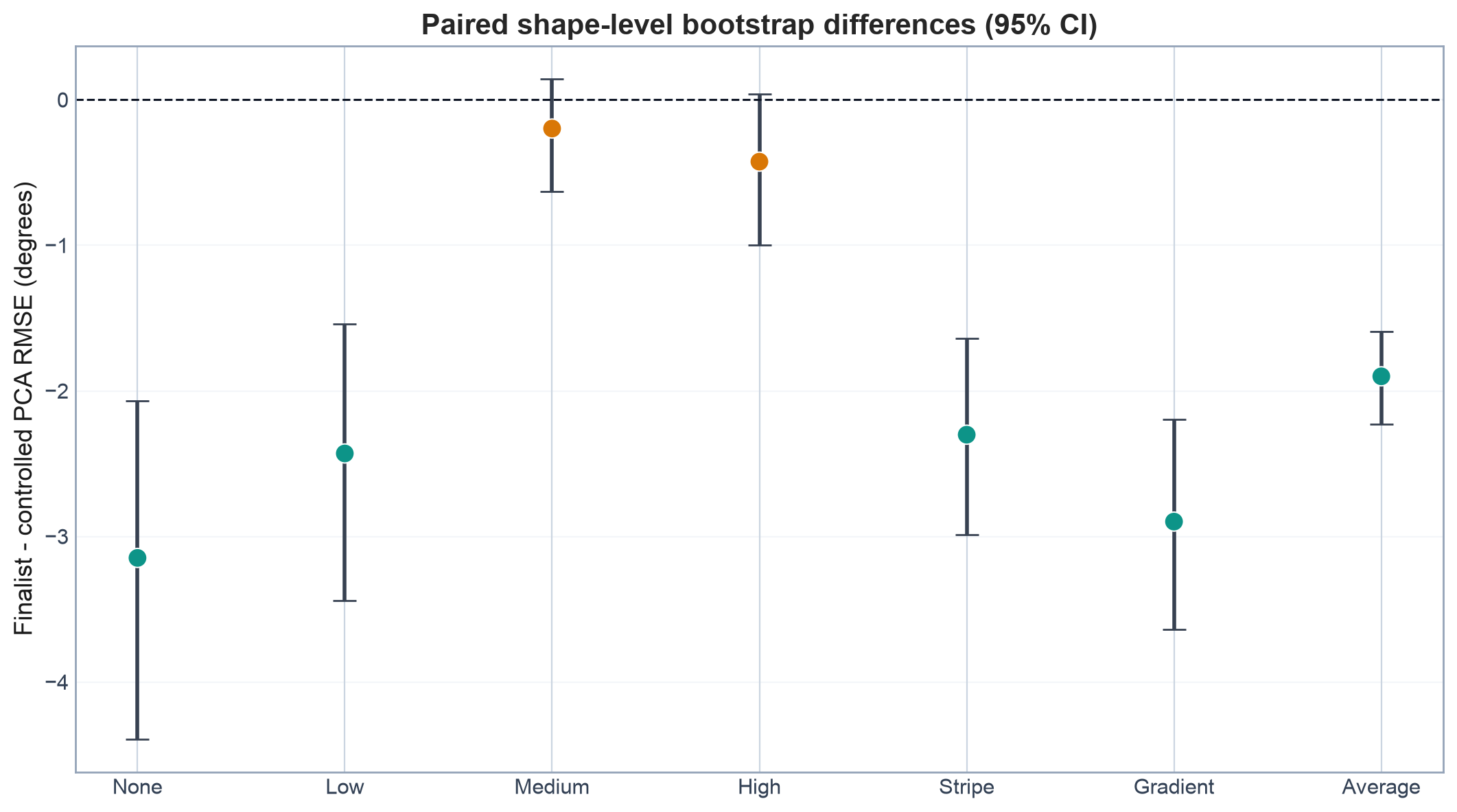
The condition-level changes are shown below.
| Condition | RMSE change | Relative reduction | 95% interval for change |
|---|---|---|---|
| None | -3.15° | 25.6% | [-4.39°, -2.07°] |
| Low noise | -2.43° | 18.9% | [-3.44°, -1.54°] |
| Medium noise | -0.20° | 1.1% | [-0.63°, 0.14°] |
| High noise | -0.42° | 1.5% | [-1.00°, 0.04°] |
| Stripe density | -2.30° | 16.9% | [-2.99°, -1.64°] |
| Gradient density | -2.90° | 22.7% | [-3.64°, -2.19°] |
The medium- and high-noise intervals include zero. The measured improvement is concentrated in clean, low-noise, stripe-density, and gradient-density data.
What the Result Says About Agentic Baseline Research
The published PCA row should not be interpreted as a deficient comparison. It is a stable, recognizable reference that makes methods comparable across papers. The experiment instead shows that stable reference values should not be confused with the practical limit of the underlying method family.
The headroom here required a sophisticated combination of simple mechanisms. Manually exploring 322 bounded alternatives, preserving every trade-off, and returning to promising parameter ranges would be tedious. Once a reliable outer loop existed, persistence became inexpensive. The agent could spend attempts on questions that usually receive little attention, such as whether robust statistics should use fewer points than the covariance, whether another refinement helps only thin sheets, or whether the last correction is systematically under-relaxed.
This is a natural role for coding agents in computational research. The human work remains concentrated in formulating the question, designing splits, preventing leakage, choosing what complexity is admissible, and interpreting the result. The loop supplies breadth and persistence after those choices become executable.
Limitations
Several constraints narrow the conclusions.
- There was no randomized run without the phased workflow, so this study does not isolate the workflow’s causal effect.
- Development and validation were consulted repeatedly across 322 attempts. The final test was protected, but the selected estimator is still the product of extensive model selection.
- The bootstrap describes variation across the finite PCPNet shape entries and does not account for uncertainty introduced by model selection.
- The final NumPy implementation took 12.99 seconds in its recorded Apple M4 Max test run, versus 2.55 seconds for controlled PCA, excluding precomputed neighbor search. It was about 5.1 times slower. These are single-run implementation measurements, not a hardware-normalized efficiency study.
- Token counts and API cost were not recorded.
- The study covers one synthetic benchmark and unoriented normals. Generalization to real scans, other computer graphics baselines, and downstream tasks remains to be tested.
Reproducing the Study
The frozen study release contains the estimator, controller, analysis notebook, and a tracked publication snapshot. The snapshot includes all 323 canonical records, aggregate and per-condition histories, controlled PCA and finalist test results, bootstrap intervals, checksums, environment metadata, and protocol notes.
The updated notebook regenerates the search, validation, condition, runtime, benchmark, uncertainty, and qualitative figures with readable typography for further analysis.
The result does not close the gap to learned state of the art. It does establish a concrete case. When a baseline has clear geometry, a protected evaluator, and enough unexplored design choices, a phased agentic research loop can uncover performance that a static comparison table does not reveal.
References
- H. Hoppe, T. DeRose, T. Duchamp, J. McDonald, and W. Stuetzle, “Surface Reconstruction from Unorganized Points”, SIGGRAPH, 1992.
- P. Guerrero, Y. Kleiman, M. Ovsjanikov, and N. J. Mitra, “PCPNet: Learning Local Shape Properties from Raw Point Clouds”, Computer Graphics Forum, 37(2), 2018.
- Y. Ben-Shabat and S. Gould, “DeepFit: 3D Surface Fitting via Neural Network Weighted Least Squares”, ECCV, 2020.
- R. Zhu et al., “AdaFit: Rethinking Learning-Based Normal Estimation on Point Clouds”, ICCV, 2021.
- K. Li et al., “GraphFit: Learning Multi-Scale Graph-Convolutional Representation for Point Cloud Normal Estimation”, ECCV, 2022.
- H. Xiu, X. Liu, W. Wang, K.-S. Kim, and M. Matsuoka, “MSECNet: Accurate and Robust Normal Estimation for 3D Point Clouds by Multi-Scale Edge Conditioning”, ACM Multimedia, 2023.
- Q. Li, H. Feng, K. Shi, Y. Gao, Y. Fang, Y.-S. Liu, and Z. Han, “PFF-Net: Patch Feature Fitting for Point Cloud Normal Estimation”, accepted by IEEE TVCG.
- Infobip, “Agentic Development Workflow”, companion repository for the CIKM 2026 Industry Day paper, 2026.
- A. Karpathy, “autoresearch”, 2026.